Probability Distribution Function For Machine Learning

In the previous part 1 blog, we discussed the basics yet essential topics of probability involved in machine learning, including deterministic and indeterministic probabilities, exclusive and exhaustive events, the definition of some famous terms, marginal, joint, and conditional probabilities, the famous Baye’s theorem and in the last we talked about the random variables. But the truth is, there is still too much left to discuss, and we will cover that in this blog. This blog is a continuation blog of the previous one, so if one finds it challenging to correlate some terminologies, we would highly recommend looking at part 1 blog.

Here, we are going to discuss,

• Probability distribution function and its types
• Functions related to the probability distribution
• Mathematical expectations and the calculation of mean and standard deviation.
• Discrete distributions: Bernoulli and Poisson’s Distribution
• Continuous distribution: Normal distribution

So let’s start without any further delay.

Probability Distribution Function

Like frequency distribution, where all the observed frequencies ( number of occurrences) that occurred as outcomes in a random experiment are listed, the Probability distribution listing probabilities of the events that happened in a random experiment. For example, suppose we are flipping a fair coin 10 times. 

• If we have to say the outcome in a frequency distribution format, we would say that 10 experiments, 7 times Heads come up, and 3 times Tails come up. 
• If we have to say the outcome in a probability distribution function format, we would say that 10 experiments, 7/10 is the probability of Heads coming up, and 3/10 is the probability of Tails coming up.

Probability Distribution defines the likelihood(probability) of possible values that a random variable can take.

Probability Distribution Function is of two types:

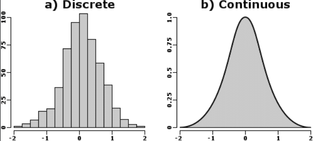
• Discrete Probability Distribution: The one with a limited number of probability values corresponding to discrete random variables.
  Ex.: Occurrence of the number of heads when a fair coin is tossed thrice.

• Continuous Probability Distribution: In this distribution, the variable can take any values in the given interval. 
  Ex.: Probability of picking a real number between 0 and 1.

Functions related to Probability Distribution:

For Discrete Probability Distribution

• Probability Mass Function (P.M.F.): PMF assigns a probability to every possible variable specific to the data attribute. If X is a discrete random variable with probabilities p1, p2, …, pn corresponding to the random variable x1, x2, …, xn, then PMF of X is given by

Would you mind observing the relation that x1, x2, …, xn are mutually exclusive and exhaustive sets for the random variable X?

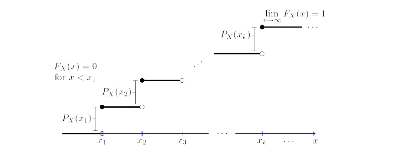
• Cumulative Distribution Function (C.D.F.): CDF assigns the same probability to the random variable x within the defined range of [Xk, Xk+1) → (including Xk and excluding Xk+1).

For Continuous Probability Distribution:

• Probability Density Function (P.D.F.): The probability of continuous variables is defined using PDF. The probability of every possible continuous value has to be greater than or equal to zero but not preferably less than or equal to 1, as a continuous value is not finite.
  Let 𝑋 is a continuous random variable then its probability density function is given by

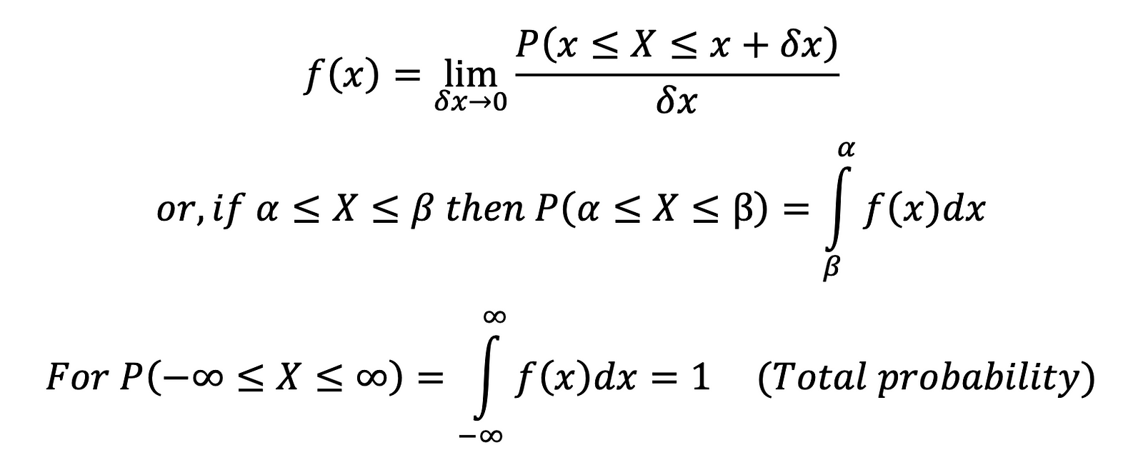
Note: In the case of a discrete random variable, the probability at any point is not equal to zero, but in the case of a continuous random variable, the probability at one fixed point is always zero, i.e., 𝑃(𝑋 = 𝑐) = 0. ( Think how? ).

Thus, we conclude that in the case of a continuous random variable,

𝑃(𝑎 ≤ 𝑋 ≤ 𝑏) = 𝑃(𝑎 < 𝑋 < 𝑏) = 𝑃(𝑎 ≤ 𝑋 < 𝑏) = 𝑃(𝑎 < 𝑋 ≤ 𝑏)

Joint Probability Distribution

If two or more random variables are given, and we want to determine the probability distribution, then joint probability distribution is used.

For Discrete random variables, Joint PMF is given by

where,

For continuous random variables, Joint PDF is given by:

Marginal Probability Distribution

If the probability distribution is defined only on a subset of variables, the marginal probability distribution is used. It is beneficial if the probability is estimated on only a specific input variable set when given the other input values.

For discrete variables, the marginal distribution function of X is

For continuous variables, the marginal distribution function of X is

Conditional Probability Distribution

Sometimes, there are cases where we have to compute the probability of an event when a different event happens. This probability distribution is termed conditional probability distribution.

For discrete random variables, the conditional distribution of X when Y is given:

For continuous variables, the conditional distribution function of X when Y is given:

Thus, it can be concluded that the conditional distribution function for any variable is equal to:

Mathematical Expectation:

The expectation is a name given to a process of averaging when a random variable is involved.

If X be a discrete random variable defined by the values 𝑥1, 𝑥2, …, 𝑥𝑛 with the corresponding probabilities 𝑝1, 𝑝2, …, 𝑝𝑛 then the expectation of X or expected value of X is given by

If X be a continuous random variable with probability density function 𝑓(𝑥), then the expected value of X or expectation of X is given by

Variance

Variance means variability of random variables. It measures the average degree to which each number is different from the mean.

Mathematically, let X be any random variable (discrete or continuous) with 𝑓(𝑥) as its PMF or PDF, then the variance of X [denoted as var(X) or 𝜎^2] is given by

Standard Deviation

Standard deviation [denoted as SD or 𝜎] is a statistic that looks at how far from the mean a group of numbers is by using the square root of the variance.

Mean (𝝁 𝒐𝒓 𝝈)

If 𝑥1, 𝑥2, …, 𝑥𝑛 are the 𝑛 variables then,

Or, if 𝑓1, 𝑓2, …, 𝑓n are the observed frequencies corresponding to the variables 𝑥1, 𝑥2, …, 𝑥𝑛 respectively then,

Probability Distribution

We know that Probability Distribution is the listing of the probabilities of the events that occurred in random experiments. Probability Distribution is of two types: i) Discrete Probability Distribution and ii) Continuous Probability Distribution.

• Discrete Probability Distribution
• Bernoulli Distribution
• Binomial Distribution
• Poisson’s Distribution
• Continuous Probability Distribution
• Normal or Gaussian Distribution

Bernoulli Distribution: The Bernoulli Distribution is a discrete distribution where the random variable 𝑋 takes only two values, 1 and 0, with probabilities 𝑝 and 𝑞 where 𝑝 + 𝑞 = 1. If 𝑋 is a discrete random variable, then 𝑋 is said to have a Bernoulli distribution if

Here 𝑋 = 0 stands for failure and 𝑋 = 1 for success.

Binomial Distribution: The Binomial Distribution is an extension of the Bernoulli Distribution. There are 𝑛 numbers of finite trails with only two possible outcomes, The Success with probability 𝑝 and The Failure with q probability. In this distribution, the probability of success or failure does not change from trail to trail, i.e., trails are statistically independent. Thus, mathematically a discrete random variable is said to be Binomial Distribution if,

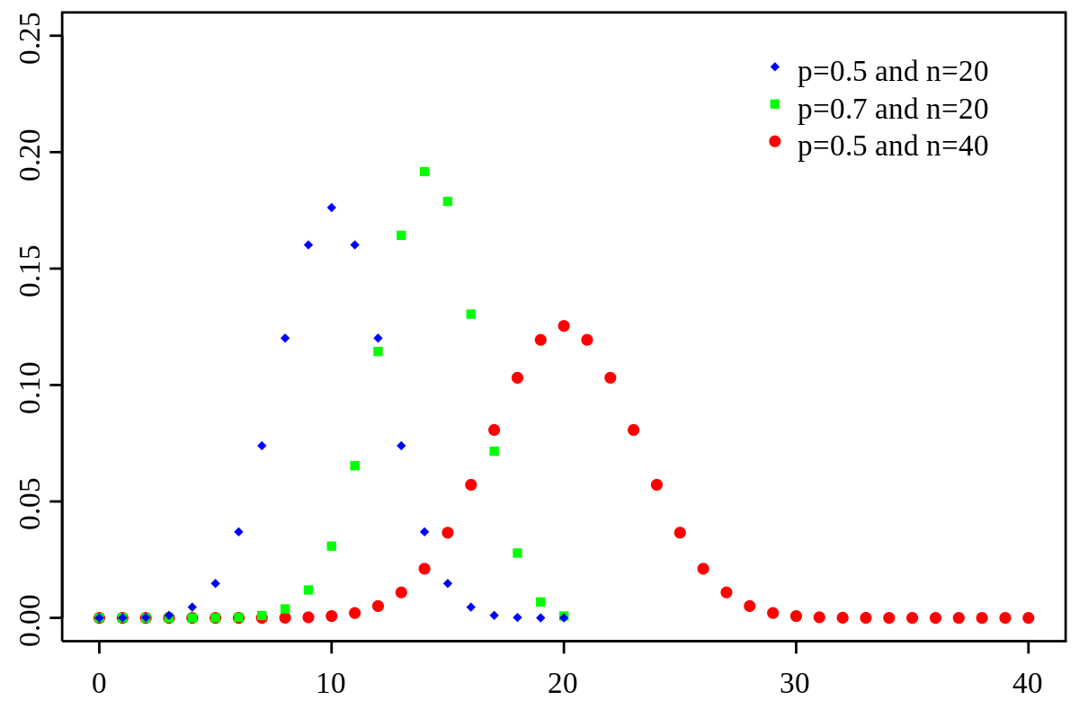
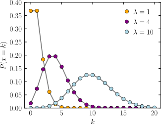
Poisson’s Distribution: The Poisson’s Distribution is a limiting case of Binomial Distribution when the trails are infinitely large, i.e., 𝑛 → ∞, 𝑝, the constant probability of success of each trail is indefinitely small, i.e., 𝑝 → 0 and the mean of Binomial distribution [𝑛𝑝 = 𝜆] is finite.

Mathematically, a random variable 𝑋 is said to be a Poisson Distribution if it assumes only non-negative values and its PMF is given by

Normal Distribution: Normal Probability Distribution is one of the most important probability distributions mainly due to two reasons:

a) It is used as a sampling distribution (extracting/creating data samples).
b) It fits many natural phenomena, including human characteristics such as height, weight, etc.

Apart from this, if we talk about the data coming from different sensors, noises present in those signals tend to follow the Gaussian/normal distribution. The Normal Distribution is a continuous probability function that describes how the values of a variable are distributed. It is a systematic distribution where most of the observations cluster around the central peak and the probabilities for values further away from the mean taper off (fade out) equally in both directions.

Mathematically it can be said that, if 𝑋 is a continuous random variable, then 𝑋 is said to have normal probability distribution if its PDF is given by

This can also be denoted by 𝑁(𝜇, 𝜎2).

When 𝜇 = 0 and 𝜎 = 1, the distribution becomes a special case called Standard Normal Distribution.

Any normal distribution can be converted into a Standard normal distribution using the formula.

Which is called ‘Standard Normal Variate’, and the 𝑍 here represents the Z-distribution. This process is also known as standardization.

Conclusion

This article was the continuation of the part 1 article on the topic of probability for machine learning. In this article, we covered the distribution function in greater detail, where we discussed the types of the distribution function, and the functions involved in the distribution function. After that, we discussed the mathematical expectation, mean, variance, and standard deviation of any probability distribution function. In the last, we discussed four primary distribution functions, including gaussian or normal distribution. We also discussed the standardization process, which is used to convert normal distribution into standard normal distribution. We hope you enjoyed the article.

Enjoy Learning! Enjoy Mathematics!